Mapping in Python - Pandas and Altair

Mapping with Python Libraries

In this module, we will repeat some of the steps of the very first tutorial, but using popular python libraries for data science and mapping, pandas, geopandas and altair.

We will be repeating all of the steps that use vector data from tutorial 1. While it is absolutely possible to work with geospatial raster data in python, this tutorial will focus on a few packages that are at home within the field of data science, and as such tend to privilege tabular datasets.

If you have not worked with any of the other tutorials that used code yet, and this is your first experience: Don't try to write everything out yourself, but rather copy them directly and try to understand the logic. It is totally ok to begin working with something that you do not totally understand, comprehension often then comes from trying to edit it.

Background

Pandas is a python library often used for data science. In programming, a library is a collection of pre-written reusable chunks of code that make writing code for specific applications easier. Pandas is written and maintained by a group of open-source contributors, and makes functionalities of python for data manipulation more accessible than they otherwise would be if one was writing in vanilla python. The key piece of pandas is the dataframe, which can be thought of as a datatype to store essentially a spreadsheet of data (meaning rows and columns). Geopandas is simply pandas but for geospatial data. They are often used in combination with eachother.

Altair is one of many libraries that allow us to make maps in python. The most popular one is matplotlib, but its syntax is a little confusing to introduce in this short module. Altair does a great job of balancing easy to read code while still being powerful and fast.

In this tutorial, we will use Google Colab to run our code. Colab is a programming environment that allows for the execution of Python code in the browser. It extends on the notebook concept pioneered by Jupyter Notebooks, and combines that with the group editing features of google docs, plus Google's cloud computing infrastructure so that all of your code is not run on your computer. We will use it here because it requires virtually no setup, but with slight modifications this code could run in any programming environment.

Instructions

Setup

Let's start by inputting this into the first cell of our colab notebook. This imports all of the libraries that we will be using.

from google.colab import files
import io

import pandas as pd
import geopandas as gpd
import altair as alt
from altair import datum

Go ahead and run the cell.

Next, let's use our datasets from tutorial 1, namely our street tree census, and our block group shapefile. To keep things simple, I exported the block groups as geopackage(.gpkg) so that we do not have to import the files that accompany the shapefile into colab. I will link to them here for convenience, but as a reminder these are subsets of the original dataset for convenience. You can find more info about these datasets (and links to the original datasets of all of nyc) in tutorial 1.

• New York City 2015 Street Tree Census
• New York City Census Blocks 2010

Step 1: Import Data

Next, paste this code below into a cell.

# upload data
uploaded = files.upload()
for fn in uploaded.keys():
  print('User uploaded file "{name}" with length {length} bytes'.format(
      name=fn, length=len(uploaded[fn])))

At this stage you should upload both of the datasets linked above. Run the cell after you copy the text, upload the first dataset. Once it is finished, do it again, and upload the second dataset. Once you are done, you will see both of your datasets in the menu accessible via the folder icon on the left

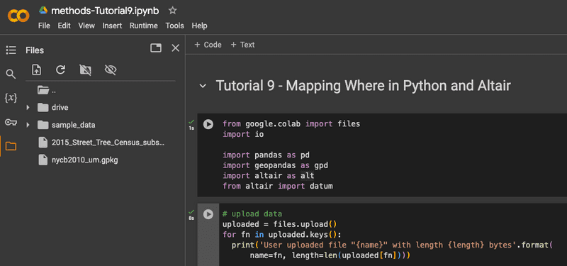
Make sure you have both files in there before you proceed, they may take a second to show up.

Step 2: Adding Street Tree Census

Now let's add our first dataset, put it into a dataframe, and check it out.

df_StreetTree = pd.read_csv('/content/2015_Street_Tree_Census_subset_um.csv')

df_StreetTree

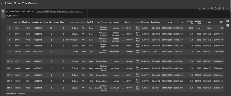
What this snippet above does is read the csv that we uploaded, and store it as a dataframe. I have named this dataframe df_StreetTree, and in general df is often used as a prefix to note which variables are dataframes. This is relevant info if you ever go on stack exchange or use an LLM (trained off stack exchange) for assistance.

When you run it, you will get a data frame like this. You can see there are 12715 rows x 45 columns (although all are not visible). By default, pandas will show you the first 5 and the last 5 rows, but you can change this.

Step 3: Mapping Street Trees

Deciding what to map

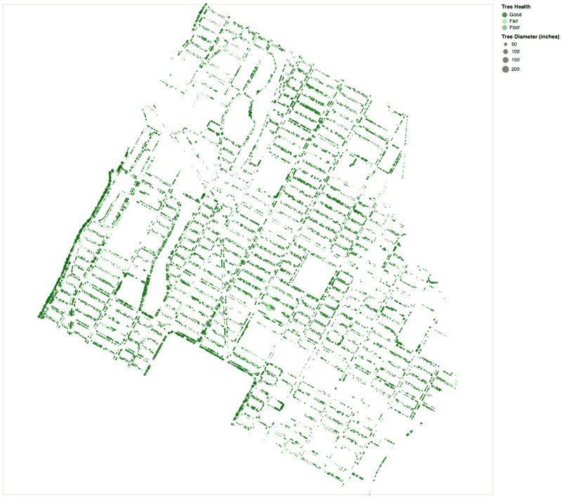
Now let's map our data. I would like to map each of the trees in our data frame with circles as we did in tutorial 1, but I would like for the color of the circles to be driven by the health (health) of tree, and for the size to be driven by the diameter at breast heigh (tree_dbh). The latter should be fairly straight forward, but in order to do the former, I need to know what the tree health values are. To do that, I will ask pandas for unique values in the health column. Copy this code and run it.

df_StreetTree['health'].unique()

Here, we have our dataframe (df_StreetTree), and are accessing the health column by putting it in brackets. Brackets signify an array of values - a one-dimensional data storage type (whereas a dataframe is two-dimensional). From there, we will use the .unique() function to see the unique values in that column. You can find more about that function in the documentation here.

The output I get says array(['Good', 'Fair', nan, 'Poor'], dtype=object).

Mapping

Now let's map it. In altair, maps are called charts, partly because they can easily be written as non-geospatial visualization methods (such as charts and graphs) as well as maps.

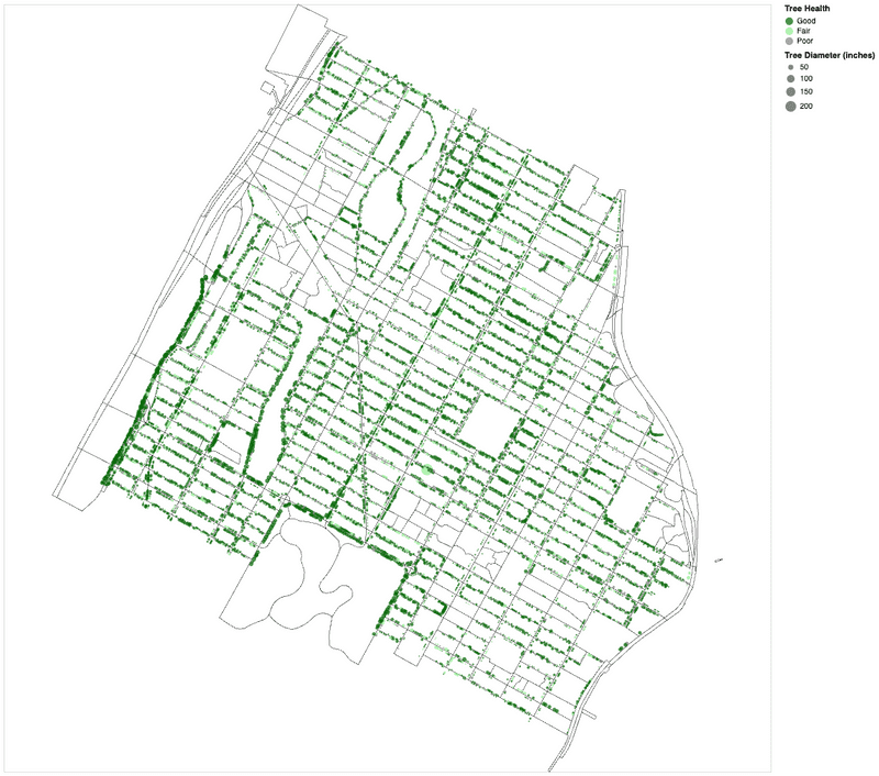
In the snippet below, I start by disabling the max rows in altair (which we are referring to with alt as defined in our import). I am doing this because by default altair will limit itself to the first 5000 rows in any dataframe. We have way more than that. Next, I define the chart with chart_StreetTree (which also saves the map with that name so we can use it again later), give it the dataframe, the symbol type (mark_circle()), the columns that contain geospatial info, data driven parameters for color and size, what the tooltip should show when the mouse hovers, and finally the projection and dimensions of the map.

alt.data_transformers.disable_max_rows()

chart_StreetTree = alt.Chart(df_StreetTree).mark_circle().encode(
    longitude='longitude:Q',
    latitude='latitude:Q',
    color=alt.Color('health:N',
                    scale=alt.Scale(domain=['Good', 'Fair', 'Poor'],
                                    range=['darkgreen', 'lightgreen', 'gray']),
                    legend=alt.Legend(title='Tree Health')),
    size=alt.Size('tree_dbh:Q',
                  scale=alt.Scale(range=[0, 228]),
                  legend=alt.Legend(title='Tree Diameter (inches)')),
    tooltip=['longitude:Q', 'latitude:Q', 'health', 'tree_dbh']
).project(
    type='mercator'
).properties(
    width=1000,
    height=1000
)

chart_StreetTree

You should end up with something like this:

Step 3: Adding and Mapping Block Group Vectors

Now let's add our Block Group TIGER Line shapefile. As a reminder, I converted this to the geopackage in the link above, this will not work if you are just uploading a singular shapefile as has been covered in this class. There are ways to work with shape files, but we'll do this way for simplicity's sake.

Copy this code and run it. Here we are uploading our geopackage, projecting it to epsg=4326, and reading it into a geo data frame, or gdf. This marks the point where we now start to use geopandas in addition to pandas. The reason why we do this now and not before is because we are working with spatial datasets, whereas csvs are simply tabular datasets, that contain information (in this case coordinates) that can be ready spatially.

gdf_BlockGroup = gpd.read_file('/content/nycb2010_um.gpkg').to_crs(epsg=4326)

gdf_BlockGroup

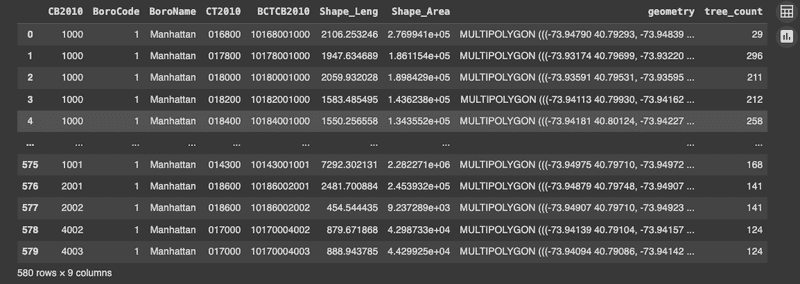
Same as before, you should see a dataframe (gdf_BlockGroup) of the dataset. You'll notice one key difference with df_StreetTree: The final column is caled geometry, and contains a multipolygon.

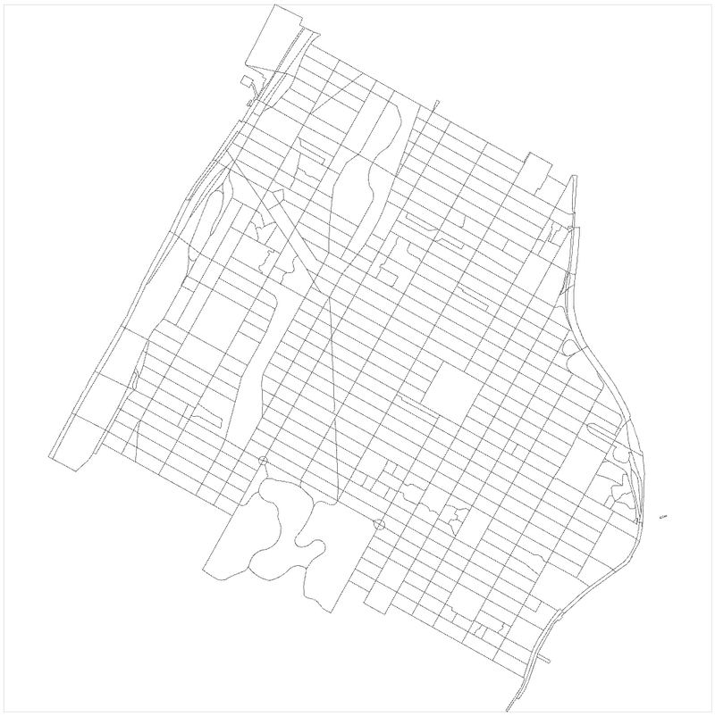
Let's go ahead and map this real quick, just white fill and black lines will do:

chart_BlockGroup = alt.Chart(gdf_BlockGroup).mark_geoshape(
    stroke='black',
    strokeWidth=0.5
).encode(
    color=alt.value('white')  # You can specify the color here or use a column from the GeoDataFrame
).project(
    type='mercator'
).properties(
    width=1000,
    height=1000
)

chart_BlockGroup

You should end up with with the map below.

One of the nice things about Altair, is that because we have been naming these charts, they are very easy to reference again later. Here we will combine the last two maps we made, simply by combining them into a new one:

combined_Chart = chart_BlockGroup + chart_StreetTree

combined_Chart

You should end up with the map below.

Step 4: Performing a Spatial Join

Now that we have our two datasets, let's perform a spatial join on them so that we can see how many trees are in each block group, the same as we did in QGIS in tutorial 1. Let's go line by line here, don't copy this code just yet:

This first line will convert our street tree dataframe into a geodataframe, by encoding the point coordinates as geometry:

gdf_StreetTree = gpd.GeoDataFrame(df_StreetTree, geometry=gpd.points_from_xy(df_StreetTree['longitude'], df_StreetTree['latitude']))

This next line will perform the spatial join itself with a function called sjoin. We will give the function are two dataframes, and specify how=right and op=contains. In order, right means that we will keep the structure of the dataframe on the right (df_StreetTrees), meaning that in the end we will have block group information joined to every row of our street tree dataset. op=contains specifies what spatial operation we want the function to use - in this case we do contains because we want all of the instances where points fall within the polygons. If we had a different geometry other than points, we may choose intersects or something else depending on the kind of information we wanted to create.

gdf_joined = gpd.sjoin(gdf_BlockGroup, gdf_StreetTree, how='right', op='contains')

After we join the datasets, we will make a new dataset out of just the block groups (CT2010), with the amount of trees in each block group (we are choosing tree_id here, but really any column would work). We're going to do this all with the groupby function.

gdf_counts = gdf_joined.groupby('CT2010')['tree_id'].count().reset_index()

The last two lines I will include with the full code. They rename tree_id to tree_count in order to describe the data better, and create a new dataframe by merging just that column back into our original BlockGroup dataframe. As a side note, we have been essentially creating new dataframes at every step instead of editing existing ones - that is just a way of working with pandas and geopandas that will result in less errors. You will notice a warning if you ever try to essentially overwrite a dataframe with an edit. It will work, but if you do it many times it could cause problems down the line.

Okay, here is the full code for joining the dataframes and printing the result. Go ahead and copy this into your programming environment.

# Convert df_StreetTree to a GeoDataFrame
gdf_StreetTree = gpd.GeoDataFrame(df_StreetTree, geometry=gpd.points_from_xy(df_StreetTree['longitude'], df_StreetTree['latitude']))

# Perform spatial join using sjoin
gdf_joined = gpd.sjoin(gdf_BlockGroup, gdf_StreetTree, how='right', op='contains')

# Group by block group and count the number of trees
gdf_counts = gdf_joined.groupby('CT2010')['tree_id'].count().reset_index()

# Rename the count column
gdf_counts.rename(columns={'tree_id': 'tree_count'}, inplace=True)

# Merge the tree counts back to the block group GeoDataFrame
gdf_TreeBlocks = gdf_BlockGroup.merge(gdf_counts, on='CT2010', how='left')

gdf_TreeBlocks

You should end up with a dataframe like below. The most important thing here is the last column, tree_count which tells us how many trees are in each block group.

Mapping our created dataset

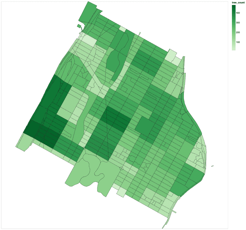
Now, let's map the result. As always let's create a new chart (chart_TreeBlocks). Here, we will use the mark_geoshape operation with Altair to style our map as choropleth. We will style a color gradient driven by the tree_count field, and mark the block group id (CT2010, feel free to rename this colum to something more descriptive first if you like) and number of trees on the tooltip. As before, we'll specify mercator and the size of the chart.

# Map the count of trees in each block group using Altair
chart_TreeBlocks = alt.Chart(gdf_TreeBlocks).mark_geoshape(
    stroke='black',
    strokeWidth=0.5
).encode(
    color=alt.Color('tree_count:Q', scale=alt.Scale(scheme='greens')),
    tooltip=['CT2010:N', 'tree_count:Q']
).project(
    type='mercator'
).properties(
    width=1000,
    height=1000
)

chart_TreeBlocks

Your resulting map should look something like this:

Final Map

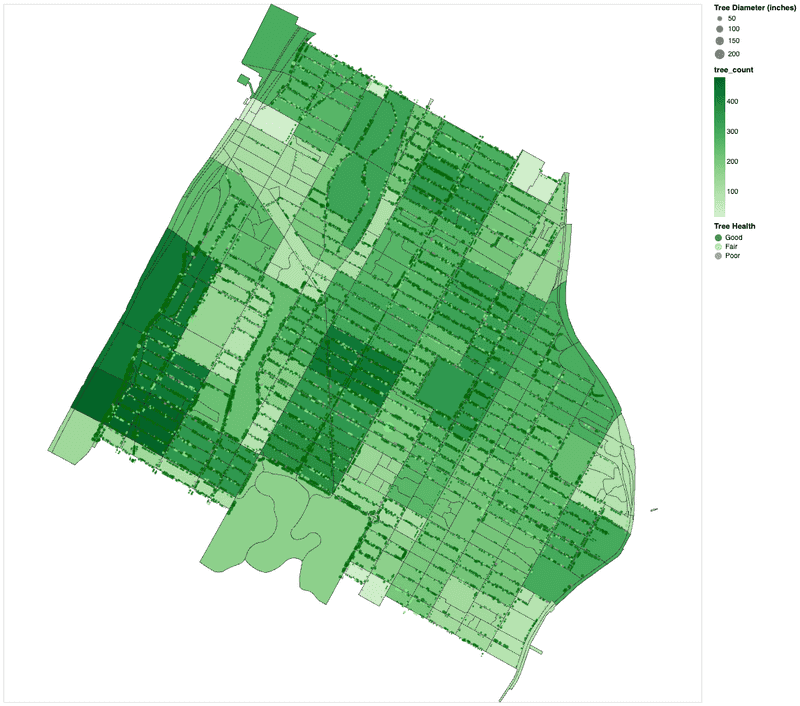
Now let's create our final map, which is just our blockgroups with amount of trees, with trees overlaid on top. For this, we can take advantage of one of the best features of altair again, which is just creating a new map by combining the saved names of the previous ones:

Final_Chart = chart_TreeBlocks + chart_StreetTree

Final_Chart

That's it! Your final map should look like this:

Challenge

Now that we have recreated a portion of Tutorial 1 in Python, for the assignment please wrangle your own data to create your own map. You can choose anything you like, but you must have at least one non-spatial dataset, and join it to a spatial one. If you are not sure of what you may choose, you could recreate tutorial 5 in your notebook (just the tutorial, not the challenge).

Module by Adam Vosburgh, Spring 2024.